Your GPU Says 100% and Your Model Still Crawls. The Real Bottleneck Is the Kernel You Never See.

I have watched a lot of training runs sit at 100% GPU utilization and still take twice as long as they should. The first few times, I did what most people do. I assumed the card was the limit, asked for a bigger one, and moved on. That was the wrong read. The card was barely working. It just looked busy.

The thing deciding your real speed is the kernel, the small program the GPU actually runs when you call something like torch.matmul. You almost never write one by hand. You pick them without knowing it, every time you set a batch size or a vocabulary size, and those picks can swing training time by 25% or more on the exact same hardware. I want to walk through what a kernel is, why your tensor shapes silently choose a fast or slow one, what the GPU spends its time waiting on, and the handful of changes that actually move the number.

Why 100% utilization is lying to you

Start with the number everyone trusts. You run nvidia-smi, the command that reports how busy your GPU is, and it says 100%. The instinct is to read that as the chip being full. It is not what the number means.

That 100% only says at least 1 kernel was running during the sampling window. NVIDIA’s own documentation defines GPU utilization as the fraction of time over the past sample period that 1 or more kernels was executing, with no account of how much of the chip each kernel used. A single kernel using a few dozen threads out of the tens of thousands a modern GPU can run will still report 100% as long as it never stops. The card looks maxed out while almost all of its math units sit idle.

So the real question underneath your step time is not whether a kernel is running. It is how much of the chip each kernel keeps busy, and how long each one waits on memory or on the CPU before it can do anything. Those are 3 separate problems, and they have 3 separate fixes.

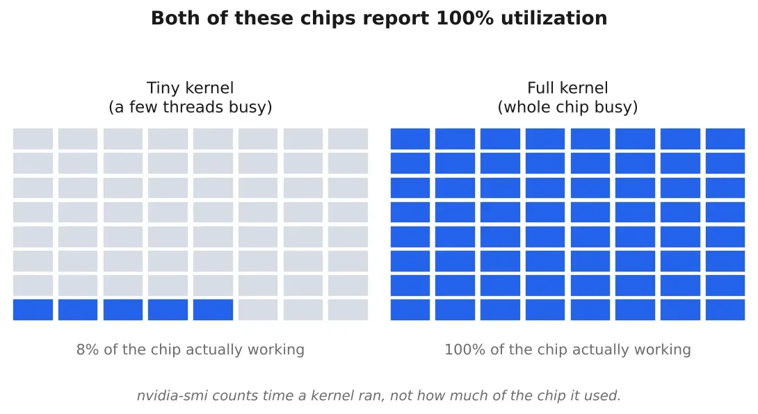
Figure 1. What nvidia-smi actually measures. A kernel using a sliver of the chip reports the same 100% as one using all of it. Source: NVIDIA System Management Interface docs

What a kernel actually is

A GPU kernel has nothing to do with the Jupyter kernel you restart when a notebook hangs. That one is the Python process running your cells. A GPU kernel is 1 small function the GPU copies across your data and runs thousands of times at once.

Each copy runs as a thread, and a GPU thread is far cheaper than a CPU thread. The GPU launches thousands of them together, each working on 1 slice of the result. Threads are grouped into blocks, and every thread reads its own index to figure out which slice it owns. A simple vector add of 2 arrays with 262,144 elements each might launch 1,024 blocks of 256 threads, which is 262,144 copies of the same tiny function, each adding 1 pair of numbers.

The GPU runs those copies on the small processors that make up the chip, which NVIDIA calls streaming multiprocessors, or SMs. Each SM has its own math cores and its own small, fast on chip memory. An A100 has 108 of these SMs. An H100 has 132, with 128 math cores each. That SM count matters more than it looks, and in a minute you will see it decide your speed directly.

Every kernel has 3 moving parts. The code is the set of steps each copy runs, identical for every thread. The launch configuration is how many blocks run and how many threads sit in each block. The data is the tensors the kernel reads out of GPU memory and the result it writes back. In plain PyTorch you touch none of that code. You choose 3 numbers instead, the batch size, the sequence length, and the vocabulary size, and PyTorch hands those to NVIDIA’s math library, which picks the kernel that runs.

The reason all of this matters, in one chart

Before the mechanics, here is the pressure behind them. Over the past 20 years the peak math throughput of accelerators grew about 3x every 2 years, roughly 60,000x in total. Memory bandwidth, the rate at which the chip can pull numbers in from its own memory, grew only about 1.6x every 2 years, roughly 100x in total. The interconnect between chips grew slower still, about 1.4x every 2 years. Those numbers come from AI and Memory Wall, a 2024 analysis by Gholami and colleagues, and they describe a widening gap. The chip can do math far faster than it can be fed.

Model size pulled in the opposite direction over the same window. The same paper measures Transformer parameter counts growing about 410x every 2 years and training compute about 750x every 2 years. So models got hungrier at a rate that dwarfs how fast memory learned to feed them. That mismatch is why so much of modern performance work is really memory work, and why a kernel that keeps every math core busy can still spend most of its time idle.

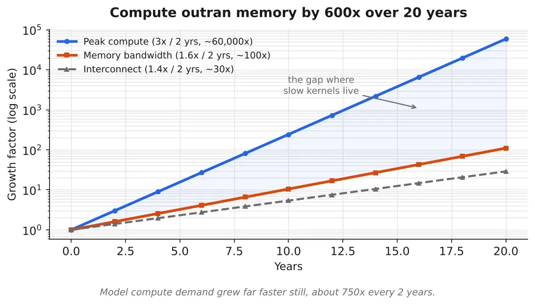
Figure 2. Over 20 years, compute grew about 60,000x while memory bandwidth grew about 100x. The gap between the 2 lines is where most slow kernels live. Source: AI and Memory Wall, Gholami et al. 2024

You can see the same gap inside a single modern GPU. An A100 does about 312 trillion 16 bit operations a second but reads from its memory at about 2 terabytes a second. An H100 pushes compute to roughly 990 trillion operations a second while bandwidth climbs only to 3.35 terabytes a second. Divide the 2 and you get a hard rule of thumb. On an A100 a kernel has to do about 150 math operations for every byte it loads to keep the math cores busy. On an H100 that number rises to about 295. Any operation below its chip’s line is limited by memory, not math, and most of the small operations in a real model fall well below it.

How your tensor shapes secretly pick a slow kernel

Here is the part that surprised me the first time I measured it. The CPU never runs a kernel. It drops the launch into a queue and keeps going, and the GPU doles the kernel’s blocks out to its SMs. Each block runs on 1 SM from start to finish, and the blocks go out in rounds. Once every SM is holding a block, the leftover blocks wait for the next round.

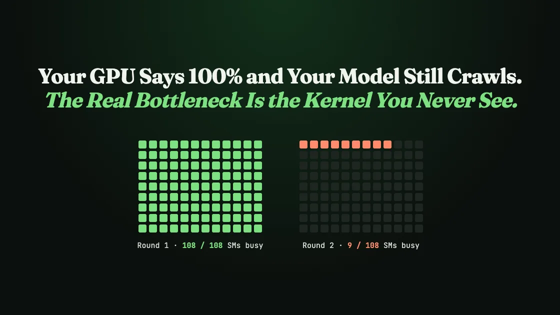
For a matrix multiply, the number of blocks comes from the shape of the result. The library slices the output into rectangles called tiles and gives each tile to 1 block. NVIDIA’s own matrix multiplication guide shows what the rounds cost on an A100 and its 108 SMs. With the library’s largest tiles, each SM handles 1 block at a time. A result that comes out exactly 12 tiles wide and 9 tiles tall is 108 tiles, which fills all 108 SMs in a single clean round. Now make that result 8 columns wider. Every row suddenly needs a 13th tile, so the launch jumps to 117 blocks. The first 108 run together in round 1, then the last 9 run alone in round 2 while 99 SMs sit completely empty. You added roughly 0.5% of extra work and nearly doubled the time. Nothing changed except the width of 1 matrix.

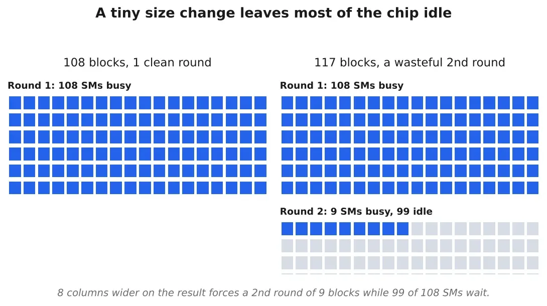
Figure 3. 117 blocks on 108 SMs. The second round carries 9 blocks and leaves 99 processors idle, so a tiny size change roughly doubles the time. This is called the tile quantization effect. Source: NVIDIA matrix multiplication performance guide

This is why your batch size, sequence length, and vocabulary size quietly decide your speed. PyTorch sends its matrix multiplies to cuBLAS, NVIDIA’s math library, and cuBLAS selects a kernel from the exact dimensions of the 2 matrices being multiplied, which those 3 numbers set. On an A100, the fastest kernels run best when the dimensions divide cleanly by 64, and odd dimensions ran slowest in NVIDIA’s own testing.

Andrej Karpathy ran straight into this in February 2023 with nanoGPT, his small GPT training repo. A language model’s final layer scores every token in its vocabulary, so the vocabulary size is 1 side of that layer’s matrix multiply. nanoGPT’s vocabulary had 50,257 entries, an awkward odd number. Karpathy padded it up to 50,304, which is 64 times 786. The 47 extra slots match no real token, so the model does about 0.09% more arithmetic, and yet training ran about 25% faster on the same GPU. In his words the padded size “goes down a different kernel path with much higher occupancy.” Higher occupancy means more of each SM stayed busy. The lesson I took from it is blunt. When you pick a vocabulary, a hidden dimension, or any size that lands inside a matrix multiply, round it up to a multiple of 64. It is free speed.

A full SM is not the same as a fast kernel

A kernel that fills all 132 SMs can still crawl, because a thread that is not computing is usually waiting on memory. This is the second of the 3 problems, and for small operations it is the dominant one.

Your tensors live in the GPU’s main memory, the separate stacks of chips next to the processors. Every kernel fetches its inputs from there and writes its results back there, and a single fetch takes hundreds of times longer than a single step of arithmetic. So a kernel that does only a little math per number it loads spends most of its life waiting for the next number to arrive.

A big matrix multiply is the good case. It reuses every value it loads across thousands of calculations, so the SMs stay fed. The small steps are the bad case, things like activation functions such as ReLU, normalization layers, and softmax. They do 2 or 3 operations per value and then sit idle until the next value shows up. The clearest measurement of this I know of comes from Data Movement Is All You Need, a 2020 study of BERT, Google’s language model. The authors found that normalization and elementwise operations were 0.2% of the total arithmetic yet consumed about 37% of the runtime of a BERT layer. Almost all of that time went to shipping data to and from memory, not to the math itself. These are called memory bound operations, and most models are full of them.

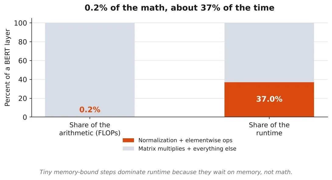
Figure 4. In a BERT layer, normalization and elementwise steps are 0.2% of the arithmetic but about 37% of the runtime. The slow part is memory traffic, not math. Source: Data Movement Is All You Need, Ivanov et al. 2020

There is a clean way to predict which case you are in before you ever run the model, and it has a name, the roofline. Take any operation and compute its arithmetic intensity, the number of math operations it does per byte it moves to and from memory. Plot that against the chip’s own ratio of peak compute to peak bandwidth, which I gave earlier as about 150 for an A100. If your operation’s intensity sits below that line, memory is your ceiling and faster math cores will not help you. If it sits above, compute is your ceiling. A large matrix multiply with big dimensions can reach hundreds or thousands of operations per byte, which is why it runs near peak. A softmax or a layer norm does a handful of operations per value, lands far below the line, and runs at a small fraction of peak no matter how expensive your GPU is. The roofline is the single most useful mental picture I have for GPU speed, because it tells you in advance whether a bigger card or a smarter kernel is the fix.

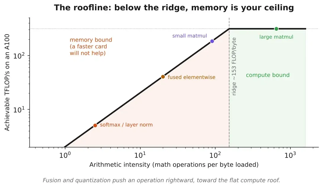
Figure 5. The roofline. An operation below the A100’s line of about 150 operations per byte is limited by memory, so a faster card does not help it. Fusion moves work rightward, toward the compute ceiling. Source: Roofline model, after Williams et al. and NVIDIA guidance

The fix is fusion, which means merging several small steps into 1 kernel so it touches memory less. Run x.cos().cos() as 2 separate kernels and they hit main memory 4 times. The first reads x, writes the intermediate result, the second reads that back, writes the final answer. Fuse them into 1 kernel and the intermediate value never leaves the chip, so only 2 trips remain and the pair runs roughly twice as fast. Plain PyTorch cannot do this on its own, because it runs 1 operation at a time and never gets to see the next one coming. The fix is a single line, model = torch.compile(model), which reads your whole model up front and fuses the chains it can. Horace He’s Making Deep Learning Go Brrrr From First Principles is the clearest explanation of why this works, and it is where I would send anyone who wants the full mental model.

The third wait is the CPU, and it hides in plain sight

The last thing a kernel waits on is Python itself. Every kernel gets launched from the CPU, 1 at a time, and Python is painfully slow next to the GPU. In the time it takes Python to add 2 numbers, an A100 can run on the order of 9 to 10 million floating point operations. A large kernel hides that lag, because the GPU is still grinding on the current one when the next launch arrives. A tiny kernel does not. It finishes before Python can hand over the next one, and the GPU goes dark in the gap.

The fix here is a CUDA graph. It records a whole sequence of kernel launches once, then replays all of them with a single launch, which deletes the per kernel Python overhead. In PyTorch you get one by passing a mode to the compiler, torch.compile(model, mode=”reduce-overhead”). Horace He’s piece has a quick test to tell whether this is even your problem. Double your batch size. If the step takes only about 10% longer, the actual work was barely costing anything and you were overhead bound, so cutting launch overhead is where your time is.

Who writes their own kernels, and what it buys them

Most of the speed work for most teams is choosing shapes and flipping on torch.compile. Writing kernels by hand is a different sport, and a few teams play it because speed is their product. Their numbers are worth seeing, because they show the ceiling.

Unsloth, an open source library for fine tuning LLMs, rewrote the model code as kernels in Triton, a Python like language for GPU code. On an A100 it fine tunes popular models around 2x faster than standard Hugging Face training while using roughly 40% to 60% less memory, with no loss in accuracy, per Hugging Face’s own benchmark writeup. If you fine tune with it, you are already running handwritten kernels.

Marlin is the kernel vLLM reaches for when a model stores its weights as 4 bit numbers, a quarter of the usual 16 bits. Shrinking the weights means a quarter of the memory traffic, and for a memory bound workload that is almost all of the cost. The Marlin paper measures the matrix multiply running about 3.9x faster than the FP16 version at batch sizes of 16 to 32, which is close to the theoretical 4x ceiling for 4 bit weights. The speedup fades as batches grow and the work turns compute bound, down to roughly 1.5x at batch 128, but near the ideal where it counts.

Cursor, the AI code editor, wrote its own MXFP8 kernels for training its mixture of experts models. Their expert layers run about 3.5x faster than the BF16 version on both the forward and backward passes, and end to end their training runs about 1.5x faster on NVIDIA’s Blackwell chips versus BF16, and about 2x faster than their old Hopper setup, all with training loss they describe as nearly indistinguishable from full precision over 10,000 steps.

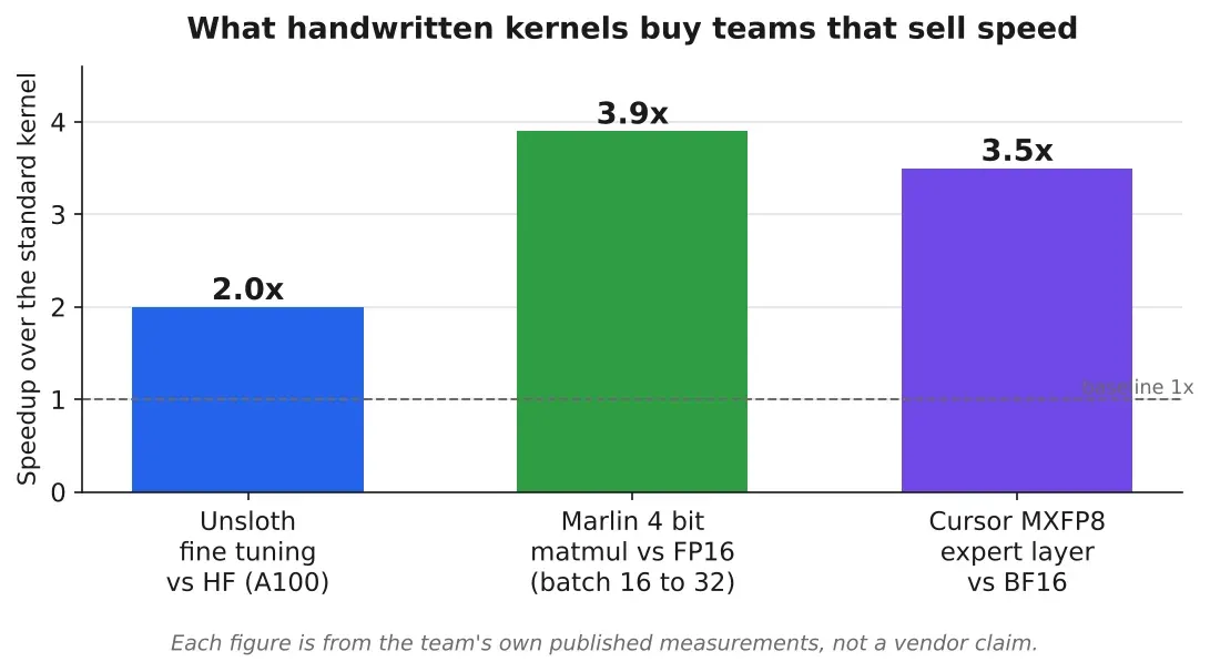
Figure 6. What handwritten kernels buy 3 teams that sell or serve at scale. Each number is from the team’s own published measurements. Source: Hugging Face, Marlin paper, Cursor engineering blog

There is also a cautionary case, and it is a good one, because it shows what a broken kernel costs when nobody is watching the output. In its postmortem of 3 overlapping bugs, Anthropic described a kernel problem inside Claude. The model picks each next token from a shortlist of the most likely candidates, which a top k kernel builds. A deployment on August 25, 2025 tripped a latent bug in the XLA compiler for TPUs, Google’s AI chips, and the approximate top k kernel began, for certain batch sizes, dropping the single highest probability token off the shortlist. The symptom was subtle quality degradation that was maddening to reproduce. Anthropic confirmed the damage on Claude Haiku 3.5, rolled that model back on September 4, and switched to an exact top k kernel, trading a little speed to guarantee the right token survived. A kernel that is fast and wrong is worse than a kernel that is slow and right.

What is oversold, and what holds up

“Write custom kernels” gets oversold for most teams. People repeat it because handwritten kernels are exactly where Unsloth, Marlin, and Cursor found their speed. But PyTorch, torch.compile, and serving engines like vLLM already ship fast kernels for the common model shapes, so for most of us the real speed work is picking good sizes and turning on the compiler. Unsloth and Cursor sell speed, and vLLM serves at enormous scale, which is why writing kernels pays off for them and usually not for you.

“The compiler will just fuse it” is half true. torch.compile merges chains of simple steps like activation functions very well. What it cannot do is invent a new way to compute something. It fuses the steps you wrote, in the order you wrote them. Attention is the operation where every token looks back at every token before it, scoring all the pairs, and the fast version, FlashAttention, exists because researchers rewrote that math so the giant intermediate score matrix never fully lands in memory. The payoff was measured, not promised. The 2022 paper reports a 15% end to end speedup on BERT large against the then standard MLPerf record, a 3x speedup training GPT-2, and 2.4x on long sequence benchmarks, all while cutting attention’s memory use from quadratic to linear in the sequence length. A compiler will not derive any of that from a naive attention loop. Someone had to rethink the algorithm so it respected the memory hierarchy, which is the whole point. The fastest kernels are the ones written by people who treated memory traffic as the real cost.

How to find your own bottleneck in 10 minutes

You do not have to guess which of the 3 waits is eating your time. Here is the sequence I run, in order, and it almost always lands on the answer.

Start with the doubling test from Horace He. Double your batch size and time 1 step. If the step gets much slower in proportion, you are compute bound or memory bound and the work is real. If it barely moves, under about 10% more time, you are overhead bound, the GPU is starving between tiny kernel launches, and torch.compile with mode “reduce-overhead” is your first move because it builds the CUDA graph that removes the gaps.

If the work is real, record a trace with PyTorch’s profiler for a few steps after the first, since the first steps burn time on 1 time setup. Open the trace and read where the time goes. A wall of small kernels named after normalization, activation, or elementwise operations means you are memory bound, and the fix is fusion through torch.compile, or a prebuilt kernel like FlashAttention for attention. A few large matrix multiply kernels dominating the time means you are compute bound, and now the shape rules pay off, so round your dimensions up to multiples of 64 and check that cuBLAS is not falling into a slow tail wave.

Serving a quantized model moves the lever again. Weights stored at 4 or 8 bits cut the memory traffic that dominates generation, so a kernel like Marlin or a serving engine like vLLM that ships one gives you most of the speed without writing anything. The order matters. Cheap settings first, profiler second, custom kernels last, and most people never need the last step.

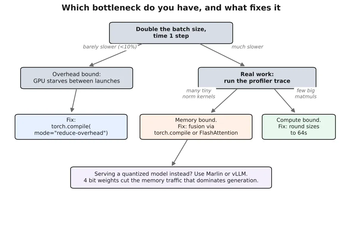
Figure 7. A decision map for the 3 bottlenecks. The doubling test and a profiler trace point you to the one fix that matters, before you spend on a bigger GPU. Source: Author’s synthesis of PyTorch and NVIDIA profiling guidance

The one habit worth keeping

You are choosing GPU kernels every time you set a batch size, a sequence length, or a vocabulary size, whether you meant to or not. Those 3 numbers decide which kernel cuBLAS runs and how many of your SMs it fills, which makes the cheapest speedup available to you a number you type in Python. Karpathy’s was a single padded vocabulary size, worth 25% faster training. Before you reach for a bigger GPU, record a trace with PyTorch’s profiler, see whether your time is going to math, to memory, or to Python, and fix the one that is actually eating your step. The card is probably faster than you think. It is just waiting.